# Never repeating, never leaving Date: 2026-07-24 Description: Four chaotic systems, one Python framework, and the one that refused to fit it. Canonical: https://shauryasharma.tech/never-repeating-never-leaving.html A strange attractor is what you get when a system is chaotic but still bounded. It never settles down to a fixed point, never falls into a repeating loop, and never flies off to infinity either. It just keeps wandering forever inside a contained region of space, tracing out a shape that has structure at every scale you zoom into. The part that took me a while to actually believe: there is no randomness anywhere in these systems. The equations are completely deterministic. Run them twice from the exact same starting point and you get the exact same path, every time. The chaos comes entirely from sensitivity to where you started. Move the initial point by a millionth and the two trajectories stay close for a while, then diverge completely. Same rules, same determinism, wildly different outcome. Edward Lorenz found the canonical example in 1963 while modeling atmospheric convection. Three coupled differential equations, nothing exotic:

\begin{matrix} \frac{d x}{d t} = σ (y - x) \\ \frac{d y}{d t} = x (ρ - z) - y \\ \frac{d z}{d t} = x y - β z \end{matrix}

With the usual constants (sigma=10, rho=28, beta=8/3), that produces output that looks like structured noise, and a shape people ended up calling the butterfly.

separation -

sigma 10.0 rho 28.0 beta 2.67

Two runs of the same equations, same constants, starting positions a millionth apart (grey and white). They ride the same lobe for a while, then peel apart onto different loops. Nothing here is random - press restart to run it again and watch it diverge differently, from the same tiny nudge. Drag sigma, rho or beta to see how the shape itself depends on the constants, not just the starting point; reset to default returns to Lorenz's own 10, 28, 8/3.

## Not building it by hand this time The last graphics thing I built was a raymarcher in plain Java, no libraries, on purpose. This project I did the opposite and reached straight for Python and a plotting library, also on purpose. The difference is what each project was actually for. With the raymarcher, the whole point was understanding the machinery, so writing my own vector math was the work, not a detour. Here, the machinery is four lines of arithmetic per system. What I actually wanted was to try a parameter, look at it, change it, and look again, fast. Writing my own 3D renderer would have been procrastination dressed up as rigor. ## Getting the first one on screen The build order was deliberately boring. Before touching any real math I plotted a throwaway spiral, just to confirm the 3D plotting pipeline worked at all. Then the Lorenz step function, sanity checked by hand on a single point. Then the integration loop, which is about as simple as numerical integration gets: ``` p = starting point repeat n_steps times: dx, dy, dz = step(p) p = p + (dx, dy, dz) * dt record p ``` That is Euler integration: take the derivative at where you are, take a small step in that direction, repeat. It accumulates error over time and there are much better methods, but for drawing a picture of an attractor it is completely fine. The butterfly showed up on the first real attempt, which felt suspicious but turned out to be true. ## The four bugs Animating it is where the actual time went. Four separate bugs, each one silent in its own way: **Axis ranges being ignored.** I set the axis ranges to stop the plot from rescaling itself, and nothing happened. In 3D figures the `xaxis`, `yaxis`, and `zaxis` settings have to be nested inside a `scene` object, not passed at the top level like they are for 2D. Passed at the top level they are silently discarded. No warning, no error, just no effect. **A redraw flag that only matters in 3D.** Animation frames have a `redraw` option that you can safely turn off for 2D scatter plots as a performance win. In a 3D scene, turning it off silently breaks the animation's progression instead. It had to be on. **A vanishing loop.** Across a few rounds of restructuring the script, the loop that actually built the trajectory kept getting lost in copy-paste. The symptom was an `IndexError` that made no sense until I checked and found my coordinate lists had exactly one point in them. The animation was faithfully trying to animate a single dot. **Frames from two attractors in one figure.** After adding a second attractor, I reused the same `frames` list without clearing it. Lorenz frames and the new attractor's frames got concatenated into one sequence, so the animation played one attractor and then abruptly cut to a completely different one in the same box. None of these threw a useful error. Every one of them just quietly did something other than what I meant. ## A second system Rössler was next. Same three-equation, same-integration-loop pattern, different arithmetic:

\begin{matrix} \frac{d x}{d t} = - y - z \\ \frac{d y}{d t} = x + a y \\ \frac{d z}{d t} = b + z (x - c) \end{matrix}

With a=0.2, b=0.2, c=5.7 it produces something visually very different from Lorenz: a single flat spiral band that winds outward, then periodically kicks up out of the plane and folds back into the middle. Lorenz has two lobes and a rough symmetry; Rössler has one band and a fold. It also needed different numbers to look right. A different step size, and roughly twice as many total steps before the folding structure becomes visible at all. That was the first hint that "how long do I run this for" is a per-system property, not a global setting. ## Making the second one boring At this point the script had two nearly identical blocks of code, one per attractor, and I was about to add a third. So I stopped and pulled out two functions. The first takes any step function at all and integrates it: ``` integrate(step_fn, initial, dt, n_steps) ``` The second takes a list of finished trajectories and renders them into one synchronized animation, side by side: ``` animate_side_by_side([(positions, title, speed), ...]) ``` The `speed` value there exists because the attractors need different step counts, but they share one animation clock. It scales how fast each one draws relative to the others, so a system that needs 40,000 steps and one that needs 10,000 can still finish at roughly the same moment. 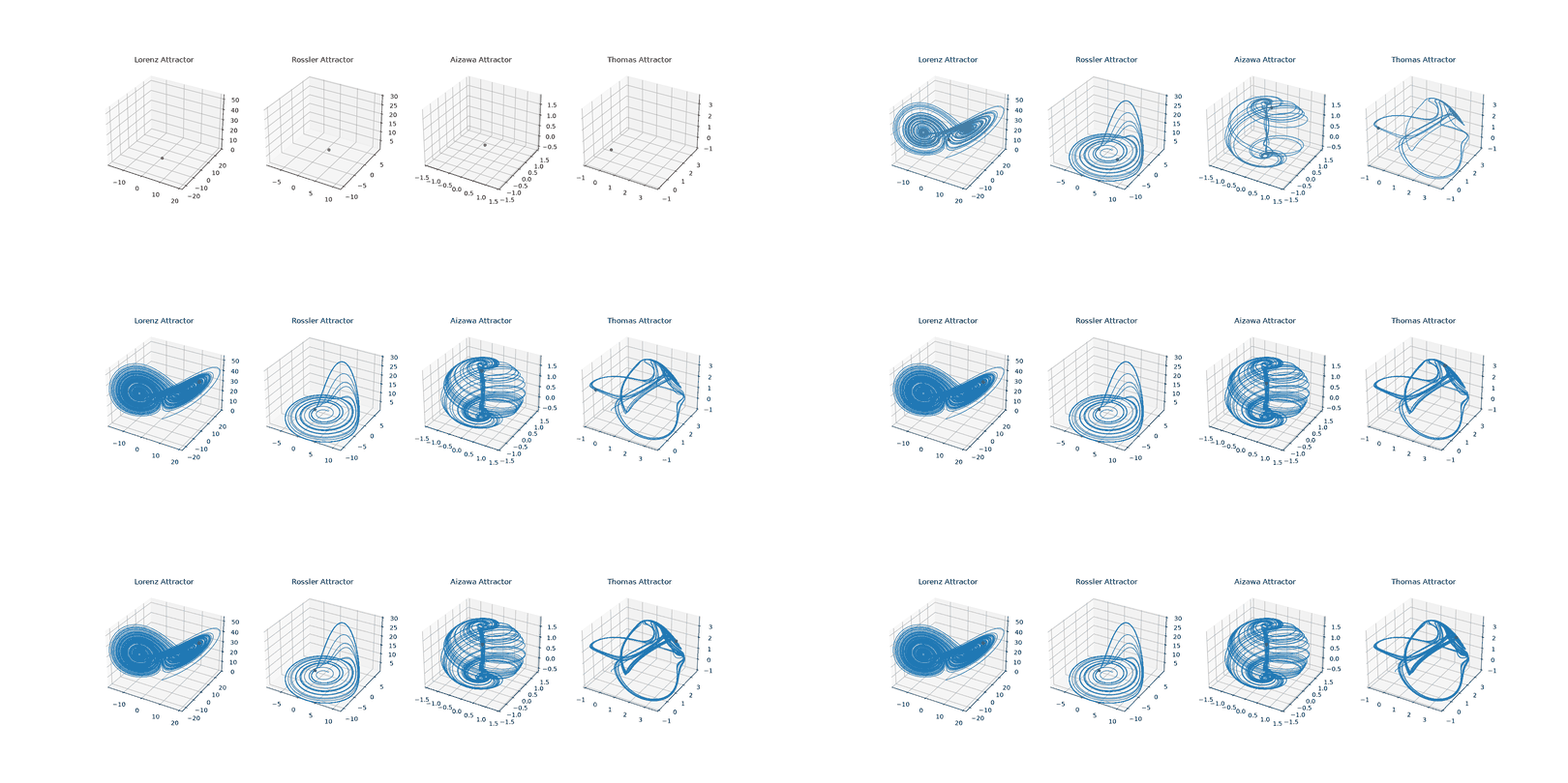The payoff was immediate. Adding Aizawa, which is a genuinely more complicated system with six parameters and a cubic term:

\begin{matrix} \frac{d x}{d t} = (z - b) x - d y \\ \frac{d y}{d t} = d x + (z - b) y \\ \frac{d z}{d t} = c + a z - \frac{z^{3}}{3} - (x^{2} + y^{2}) (1 + e z) + f z x^{3} \end{matrix}

took one new step function and one new line in a list. Zero changes to anything structural. It produces a layered, shell-like spiral that looks like something turned on a lathe.

Four 3D plots side by side, each tracing out a different strange attractor as an animated line: Lorenz's two-lobe butterfly, Rossler's single folded band, Aizawa's layered shell, and Thomas's rounded looping form. — Four systems, one framework, one animation clock. Lorenz, Rössler, Aizawa, Thomas.

## Then one of them refused to fit Clifford is where the framework stopped working, and understanding why was the most interesting part of the whole project. Everything so far has been a continuous system. There is a smooth path through space, and consecutive points along it are close together. That is exactly why animating a dot tracing a connected line makes sense as a way to show it, and why `dt` means anything at all. Clifford is a discrete map: ``` x' = sin(a*y) + c*cos(a*x) y' = sin(b*x) + d*cos(b*y) ``` There is no derivative here and no time step. You take a point, apply the formula, and get the next point, which can land anywhere in the plane. Consecutive points are not neighbours. There is no path. Drawing a line between them would be drawing a relationship that does not exist. 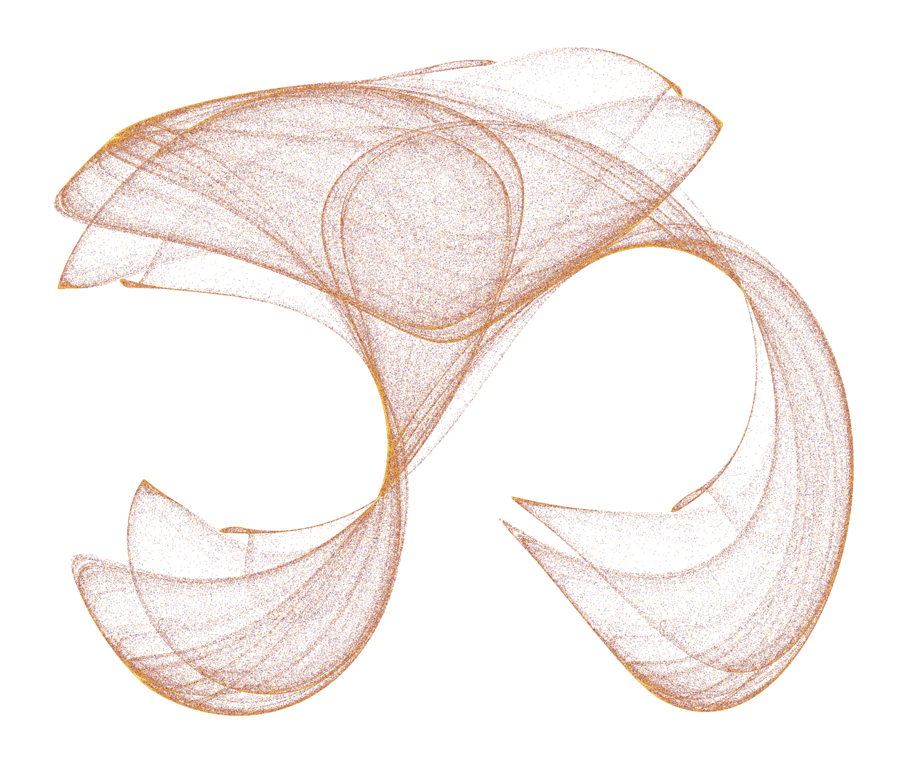So the attractor's shape does not emerge from following a trajectory. It emerges statistically, from plotting hundreds of thousands of points and seeing where they pile up. Some regions get visited constantly and go dense, others almost never. I rendered half a million iterations as a single static scatter, coloured by iteration order:

A dense static scatter plot of the Clifford attractor, forming sweeping curved bands and lobes that look like folded ribbons. — The Clifford attractor. No animation, no path, no dt. Half a million points, and the shape is what the density does.

Same word, "attractor", genuinely different object. It needed its own render path, and no amount of framework design would have prevented that, because the difference is mathematical, not architectural. ## Coda Thomas' cyclically symmetric attractor went in last, and it went back to being boring in the good way. One parameter, and unusually for this group, it is built from trigonometric functions rather than polynomials:

\begin{matrix} \frac{d x}{d t} = \sin (y) - b x \\ \frac{d y}{d t} = \sin (z) - b y \\ \frac{d z}{d t} = \sin (x) - b z \end{matrix}

With b=0.208186 it gives a softer, more rounded kind of chaos than the others. It also evolves much more slowly, so it needed a step size five times larger than Lorenz's and about four times as many steps. Two numbers and one line, no structural changes. One practical thing worth writing down: going from three panels to four made rendering the animation noticeably slower, in a way the interactive version never was. Once you export to a GIF, every frame has to be rasterized and encoded up front, so frame count is a direct multiplier on render time. The lever for that is how many simulation steps you skip between captured frames. Playback speed is set separately, so skipping more does not make the result look choppier, it just means fewer frames to build. Going from four panels back down to a reasonable render time was a one-number change. The whole thing is about 130 lines now, and adding a fifth continuous attractor would be maybe six of them. ## Further reading The source is on GitHub: [Shaurya-34/strange_attractors](https://github.com/Shaurya-34/strange_attractors).