# grok.....grok ?
Date: 2026-07-20
Description: What happens when you push a model past generalization? Does it know the rule, or just the data?
Canonical: https://shauryasharma.tech/grok-grok.html
There's a strange thing neural networks sometimes do called grokking. You train a
network on some task, and for a long time it looks basically done: the loss on
its training data has already hit zero, and nothing seems to be happening. Then,
often thousands of steps later, with no warning, its performance on data it
hasn't seen suddenly jumps. It goes from failing to almost perfect, quickly, long
after you'd have stopped watching.
The question I got stuck on was: when that jump happens, has the network found
the actual underlying rule, the real law behind the data? Or has it just found a
slightly better guess that happens to work well near the examples it was trained
on? Those sound similar but they're not. A model that found the real rule should
work anywhere, even far outside the range it was trained on. A model that found
a good local guess should fail once you move away from that range. Nobody
seemed to have actually tested this directly, and it felt like a real gap: if
grokking really does mean "found the true law," that's a big deal for any field
where you can't just go measure the thing you're predicting (drug interactions
you haven't run, materials that don't exist yet, physics at conditions no lab can
reach). If it doesn't, that's worth knowing too.
So that became the plan: pick something with an actual, known ground-truth law,
grok a model on it, and then test whether it extrapolates. I called the project
Wedge 1.
## What I already had lying around
Before starting from scratch, I checked an older project of mine called
catapult (named after [gwern's LLM catapult hypothesis](https://gwern.net/llm-catapult),
which is what got me interested in this whole area in the first place), which
had spent a while reproducing grokking on the classic toy example: modular
addition. Feed a network pairs of numbers and their sum modulo
some prime, hold out a chunk of the pairs, and watch what happens as it trains.
It turned out I'd already done a lot more with this than I remembered.
epoch -train -val -
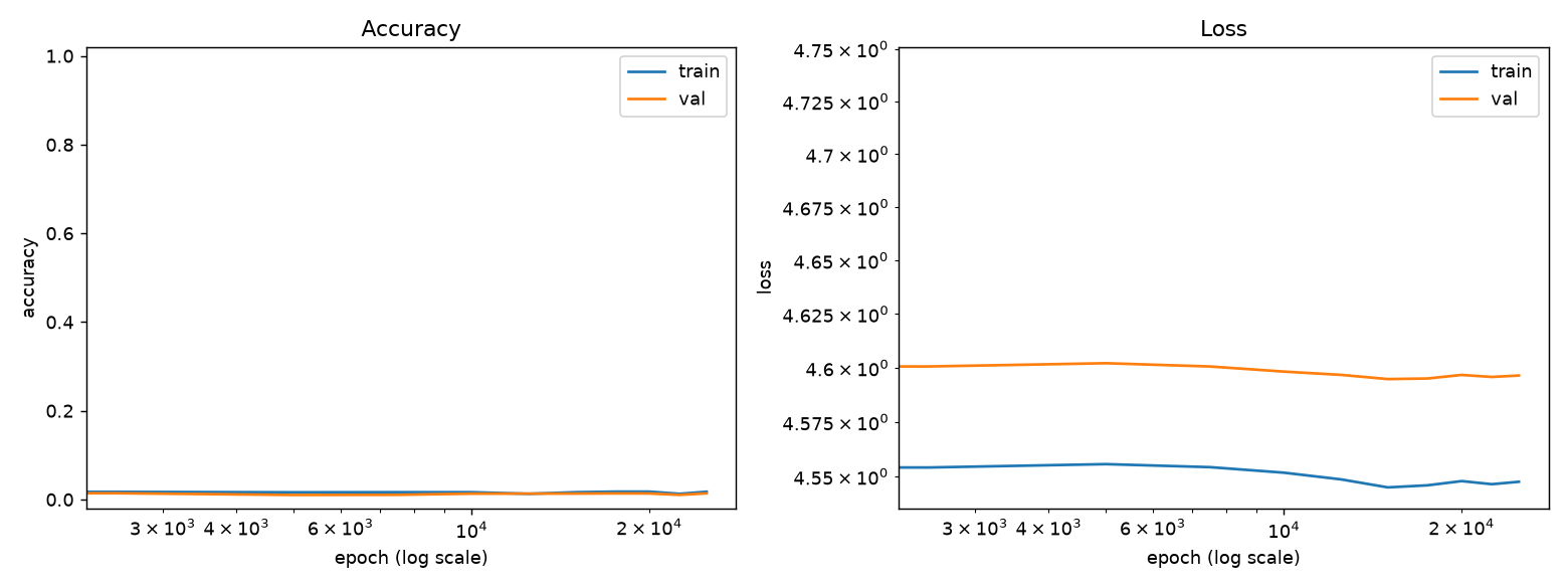
Modular addition, seed 0. Training accuracy hits 100% within 1,000 epochs; validation sits flat for thousands more, then jumps to 100%. Switch weight decay off and the jump never arrives - validation never passes 12%. Drag the slider to scrub through training.
A few things from catapult turned out to matter a lot later. First, weight decayA training setting that gently penalizes the network for having large internal numbers. wasn't optional here: turn it off and the jump in the figure above
never happens at all. Second, I could actually look inside the grokked network
and see what it was doing, not just that it worked.
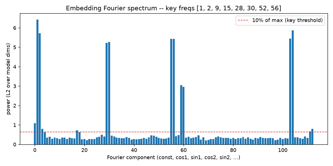
The grokked network's internal representation, broken into frequencies. A handful of sharp spikes, not noise. It's not memorizing input-output pairs, it's computing with a small set of frequencies, the same trick you'd use to do modular arithmetic with sine and cosine waves.
The trick itself is neat. Map each number onto an angle on a circle, and
adding two numbers mod p turns into adding two angles. There's a plain
trig identity for that:
which a network can compute with nothing more exotic than multiplication
and addition. Those sharp spikes in the spectrum are the fingerprint of a
network that settled on a small handful of these angles, instead of
memorizing every pair by hand.
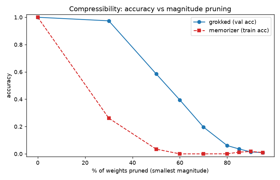
And when I compared a grokked network against one that had only memorized the
training examples, the grokked one was just sturdier in every way I tried to
break it.
Cut the smallest 30% of the network's weights and the grokked model barely notices, still around 97% accurate. Do the same to a model that only memorized the training set and it falls apart. Whatever grokking builds is more redundant, more real, than what memorization leaves behind.
I even tried to break a grokked solution back down on purpose: crank up weight
decay further, remove it entirely partway through, add noise to the labels. None
of it worked.
Trying to unlearn a grokked solution, several different ways. Once the network finds the real algorithm for modular addition, it does not let go.
So going in, I had good reason to believe grokking finds something real and
stable, at least for this kind of task. What I hadn't tested was the actual
question: does that "something real" generalize to inputs way outside the
training range. Modular arithmetic doesn't really have an "outside the range,"
so I needed a different kind of problem to test that.
## Building the actual test
For Wedge 1 I switched to physics: functions with a known, exact formula, where
I could train a network on one range of inputs and then check its predictions
somewhere it had never seen. Lennard-Jones potential was the main one, which
describes how atoms attract and repel depending on distance:
Two terms: one repulsive (`r^-12`, wins up close), one attractive (`r^-6`,
wins further out), and two positive constants that just set the strength and
scale. I also tried a couple of other shapes for variety, mostly to check
that nothing I found was specific to this one formula.
The plan was simple on paper: train a small neural network to predict the
potential from the distance, using weight decay, wait for it to grok, then
compare its predictions inside the training range against its predictions
outside it. I set the outside-the-range boundaries in advance, before running
anything, so I couldn't quietly move the goalposts later if the results looked
bad.
## Smooth functions don't grok
The first run didn't grok at all. Not "grokked slowly," not "grokked weakly."
Nothing like the sudden jump from before ever showed up.
The reason turned out to be almost embarrassingly simple. Grokking is
interesting because there's a hard gap between "memorized the training
examples" and "found the general rule," and the network sits stuck on the wrong
side of that gap for a while before crossing it. Modular addition has that gap:
you either know the rule or you're stuck guessing. A smooth physical curve
doesn't. If I show a network sixty points sampled from a smooth curve, it can
fit a curve that passes near all sixty points almost immediately, using nothing
smarter than "connect the dots." There's no hard problem for weight decay to
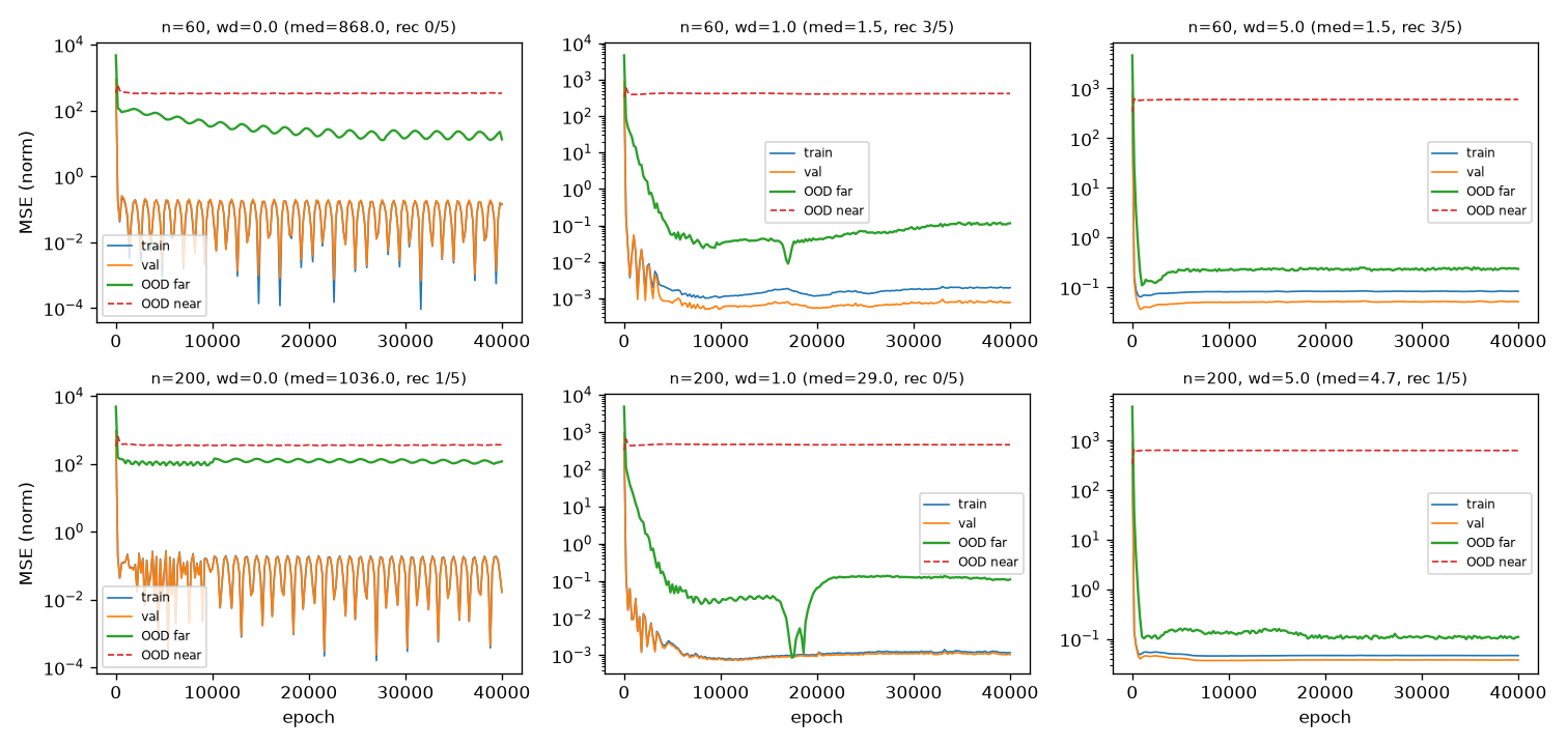
eventually solve, so there's no delayed jump. Training and validation error just
went down together, smoothly, from the start, in every setting I tried.
That also meant the plan itself was slightly wrong. I'd been asking "did this
network grok yet," but for a smooth function that question doesn't really apply.
The question that actually mattered was more direct: does the network's error
on the far-outside-the-range points improve late, well after its error on the
training range has already flattened out. That's the real signature I was
actually looking for, and I hadn't been measuring it directly.
## The long, noisy middle
Once I started tracking the outside-the-range error properly, I spent a good
while chasing what looked like real signals that turned out to be measurement
problems instead. A few examples, because I think the mistakes are more
instructive than the parts that worked:
One early "positive" result turned out to be driven by runs where weight decay
was set to zero, which makes no sense since weight decay is the entire proposed
mechanism. The actual cause was an unstable learning rate making the validation
curve jump around, which was fooling a naive "did it improve" detector into
counting noise as a signal.
Another run seemed to show the effect appearing and then not appearing,
depending on how I averaged two different failure regions together. Lennard-
Jones has a smooth, learnable far tail and also a sharp, physically extreme wall
close to zero. That near-wall region is essentially impossible to predict from
training data that never showed anything like it. Averaging it in with the
learnable far region was hiding whatever was actually going on in the part that
should have been learnable.
A later run gave a table where adding more training data made the results look
worse, which is backwards. That one came down to using a ratio (error near the
boundary divided by error inside the training range) instead of a plain error
number. With more data, the inside-the-range error got so tiny that even a small
outside-the-range error produced a huge ratio, just from the denominator
shrinking. The model wasn't doing worse. The yardstick was broken.
Each of these took real time to track down, and each time the fix was the same
kind of lesson: measure the thing you actually care about, in units that don't
lie to you, and don't trust a result until you've asked why it looks the way it
does.
## The real answer
Once the metric was fixed (comparing the network's outside-the-range error
against how much that region's true values vary, essentially asking "did this
beat just predicting the average"), the honest result was clear and not close.
A plain neural network trained on Lennard-Jones data, tested past its training window (shaded). Inside the window it tracks the true curve closely. A short distance outside it, the prediction goes flat or drifts off in a straight line while the real curve keeps bending.
Even in the best setting, the network's predictions outside the training range
were roughly 190 times worse than simply guessing the region's average value.
No amount of weight decay, however I tuned it, produced a network that had
actually recovered the true underlying formula.
The reason is almost mechanical rather than mysterious. A network built from
ReLU activations can only ever draw straight-line segments, joined together at
kinks. Inside its training window, it can fake a smooth curve by using enough
tiny straight segments that you can't see the joints. Outside the window,
though, there's no more data telling it where the next kink should go, so it
just keeps going in whatever straight line it was already on. The true physical
law keeps curving. The network structurally cannot. This isn't a training bug
you can fix with a better recipe. It's a property of what that kind of network
is.
I did wonder whether a different activation function would sidestep this, and
it wouldn't have, for the same underlying reason: smooth alternatives extrapolate
as their own shape (flat, wavy, whatever their formula naturally does far from
the data), not as the specific shape of Lennard-Jones or any other particular
physical law. Fixing this needed a different kind of change entirely.
## Changing the question
If the problem is that the network has to invent its own extrapolation shape,
the fix is to stop making it invent one. Instead of a free-form network, I built
a fixed menu of candidate ingredients, things like different powers of distance
and different exponential decay rates, and let a plain linear model choose how
much of each ingredient to use:
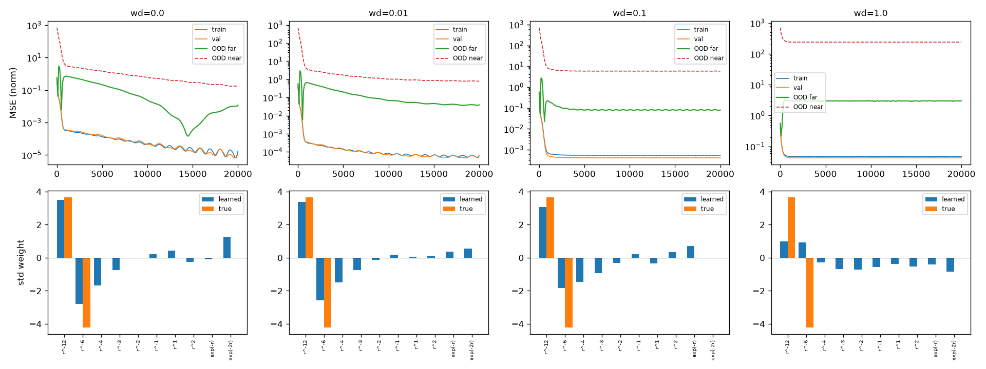
Each `f` is one menu item (`r^-12`, `r^-6`, `r^-4`, `exp(-r)`, and so on), and
each `w` is a weight the model is free to learn. The true Lennard-Jones
formula is exactly two of those ingredients: nonzero weight on `r^-12` and
`r^-6`, zero everywhere else. Everything else on the menu is a decoy that only
helps fit the training window without meaning anything.
This turns "did the model find the true law" into a question you can actually
answer cleanly: among every combination of ingredients that fits the training
data equally well, does training push the model toward the two real ones and
away from the decoys, or toward some messy mixture that only happens to work
inside the window?
The first result validated the whole idea. With the right ingredients available,
the near-wall region (previously unlearnable) got recovered almost exactly, just
because the model finally had access to the right shape. But there was a twist
I didn't expect.
Same setup, but the model can only choose from a fixed menu of physics-shaped ingredients. Turning weight decay up, the exact ingredient behind grokking, made recovery of the true two terms worse, not better.
The true answer here needs `w` on `r^-12` and `r^-6` to be genuinely large.
Weight decay's entire job is to discourage large numbers. So the stronger I
turned it up, the harder it pushed against the actual correct answer, shrinking
the true terms and leaking their weight onto decoys instead. The mechanism that
causes grokking on modular addition was actively fighting law-recovery here.
## L1 versus L2
Weight decay is what's called an L2 penaltySpreads a small tax evenly across every number in the model - shrinks everything a little rather than picking winners.: it spreads a small tax evenly
across every number in the model. There's a different kind of penalty, L1Pushes weak ingredients all the way to zero and leaves a few strong ones alone, rather than taxing everything equally.,
that behaves completely differently: instead of taxing everything a little, it
tends to push weak ingredients all the way to zero and leave a few strong ones
alone. If the true answer really is "two ingredients, and nothing else
matters," L1 seemed like the more honest tool for finding it. So I ran the
direct comparison.
Same test, L1 against L2. A light L1 penalty finds the true two ingredients almost exactly and zeroes out everything else. L2, the actual mechanism behind grokking, never gets there, and gets worse the harder it's pushed.
This was the clean result I'd been chasing, just not the one I expected. A weak
L1 penalty recovered the true law almost perfectly. Weight decay, the specific
ingredient responsible for grokking in the first place, did not, at any strength
I tried. Push L1 too hard and it also failed, wiping out the true signal along
with the decoys, so there's a real sweet spot rather than "more sparsity is
always better." But within that sweet spot, sparsity worked and grokking's own
mechanism didn't.
## So, was it worth it
At some point I asked myself directly whether any of this was actually worth
finishing, and I think the honest answer is no, not really, not as originally
framed.
The whole premise was "grokking might mean the model found the true law." But
by the time I got a clean result, that premise had already quietly stopped
being true two pivots earlier: grokking, at least as I'd studied it, is a
phenomenon about matching your training distribution well, not about reaching
beyond it. The smooth-function experiments never grokked in the first place.
What I ended up with, stripped of the physics dressing, is close to a decades-
old statistics result: L1 penalties (LASSO) find sparse answers better than L2
penalties (ridge regression) when the true answer actually is sparse. That's
real, but it's not new, and recovering a formula after handing the model its
exact ingredients in advance isn't genuine scientific discovery either. Tools
built specifically for that (symbolic regression methods that search for a
formula without being told its shape ahead of time) already do the real version
of this, and do it better.
What I do think was worth keeping is the actual path there, and specifically
the parts that were wrong at first. Overparameterizing a model isn't enough by
itself to cause grokking. Grokking, at least in every case I tested it, is
about generalizing within your training distribution, not about extrapolating
past it. A ReLU network structurally cannot bend the way a real curved law
bends outside its training data, no matter how you train it. And a metric that
measures relative error can quietly lie to you the moment your target region is
nearly flat. Those are small, useful things to actually know, and I wouldn't
have known any of them without running into each one directly.
One loose end, left exactly as it is: I'd written an improved version of the
L1-versus-L2 comparison, with a cleaner error metric and a finer sweep around
the sparsity sweet spot, but never got around to actually running it before
deciding to close the project. The result above stands on the coarser run.
That's a real gap, not a rounding error, and I'd rather say so than quietly
smooth it over.
Mostly, though, the useful part of this whole detour was just noticing the
premise had failed, and stopping instead of grinding on. That's a less
satisfying ending than a paper. It's still the right one.
## Further reading
[gwern.net/llm-catapult](https://gwern.net/llm-catapult): the original
hypothesis this whole detour, and catapult's name, borrows from.